1. Literature
| # | Title | Category | Description |
|---|---|---|---|
| 1 | MATLAB/Simulinkによる現代制御入門 | Universal | Lyapunov in Chap. 7, pp. 140 |
| 2 | Multi-objective filter design for uncertain stochastic time-delay systems.pdf | Exponentially stable | Exponentially stable lemma in page 3, pp. 151, lemma 1 |
| 3 | Observers for Nonlinear Stochastic Systems.pdf | Exponentially stable | The origin of lemma 1 of LIT#2 |
| 4 | Basic Lyapunov theory.pdf | Properties | GAS, stability theorems (exponential), Lasalle's theorem, candidate |
| 5 | Lyapunov Stability Theory.pdf | Exponentially stable | Exponential stability based on state in page 3, Exponential stability theorem based on Lyapunov functional in page 6 |
| 6 | Basic Concepts of Stability Theory | Stability | A tutorial help understanding Lyapunov stability |
| 7 | Equilibrium Points of Linear Autonomous Systems | Universal | Types of equilibrium points, phase portrait, especially for singular transition matrix |
| 8 | Method of Lyapunov Functions | Trajectory | * help understanding phase trajectory, derivatives, monotonicity |
| 9 | Nonlinear Systems (3rd Edition).pdf | ROA | Region of Attraction in pp.312 |
| 10 | MATLAB/Simulinkと実機で学ぶ制御工学 | Experiment | Experiment platform based on lego NXT |
| 11 | Making an Inverted Pendulum using LEGO MINDSTORMS EV3 | Experiment | Another experiment platform based on lego EV3 |
| 12 | 台車の振幅制限を考慮した倒立振子の安定化制御 | ROA | Calculation of ROA boundary |
| 13 | Exact Asymptotic Stability Analysis and Region-of-Attraction Estimation for Nonlinear Systems | ROA | |
| 14 | Nonlinear Systems and Control Lecture # 11 Exponential Stability & Region of Attraction | ROA | Curriculum slides of Michigan State University |
| 15 | Lasalle 不変原理による 2 次系の漸近安定性の証明 | Asymptotical stability | |
| 16 | Riccati & Lyapunov equations | LQR | Riccati LQR and Lyapunov theory |
| 17 | Markov過程の量子化を用いたLyapunov関数の構築 | Quantum | |
| 18 | Quantum stochastic calculus | Quantum | |
| 19 | Itô's lemma | Quantum |
2. Point
• Lypunov Stability: Asymptotical, Exponential
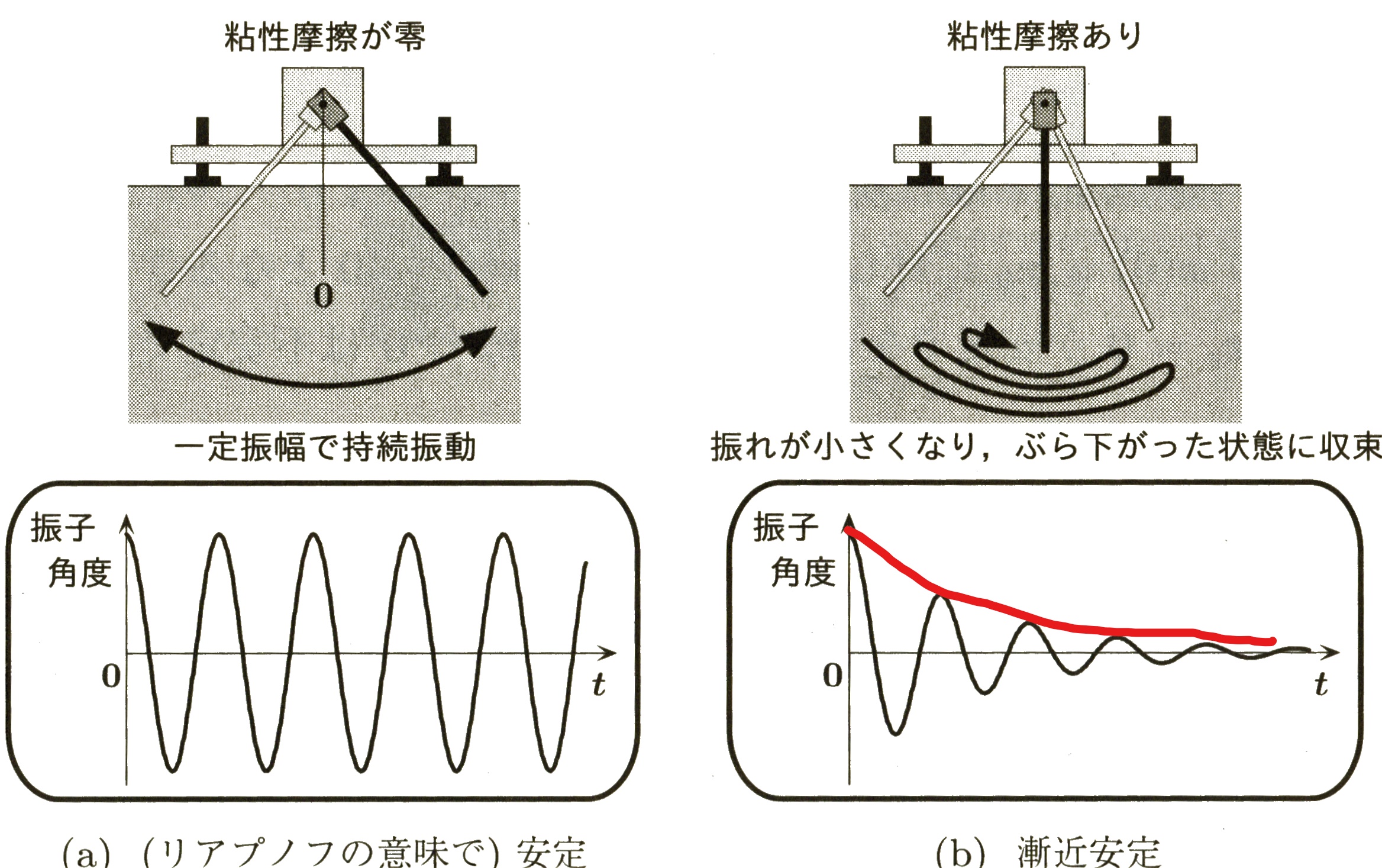
For general non-linear zero input system ([LIT 1] pp. 141)
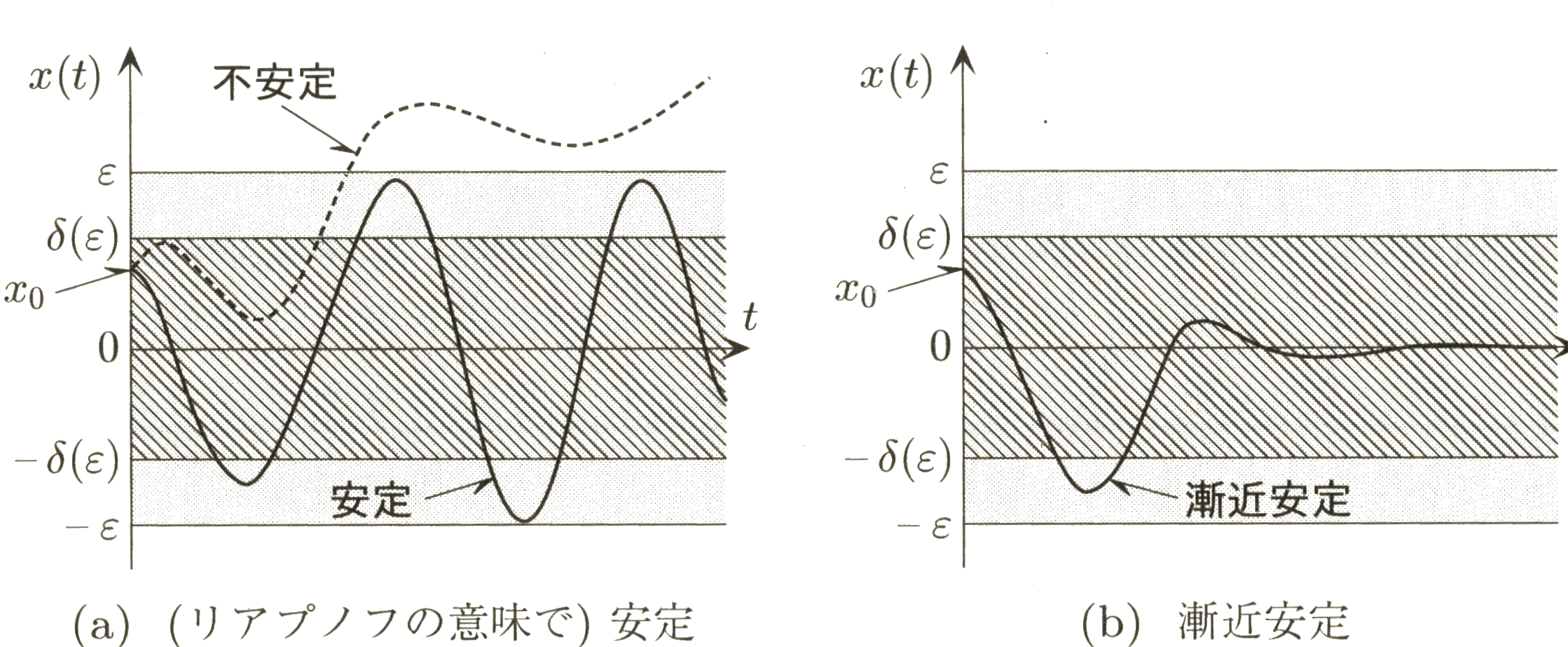
Figure 2 Lyapunov stability
The equilibrium point of equation (1) is . As is shown in Figure 2(a) , for any , there exists (no matter how small it is), when , for any time , , equilibrium point is stable. More generally [ref] , as is shown in Figure 3 ,
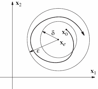
Figure 3 Lyapunov stability in 2-dimensional phase diagram
when
, there is
, furthermore, if
, then
equilibrium point
is
asymptotically stable
(
Figure 2(b)
)
. Even furthermore, if
, for
, system
equation (1)
is called
asymptotically stable in the large
or
globally asymptotically stable
(GAS) at
equilibrium point
.
Even even furthermore, if
envelop
(
red curve as is shown in
Figure 1(b)
) of
converge is at exponential rate, then the system
equation (1)
is called
exponentially stable
. (Lemma 1
[LIT#2]
,
[LIT#3]
)

Figure 4 Relation of Lyapunov stability, asymptotically stable and exponentially stable
EXAMPLE: Energy and stability of pendulum system
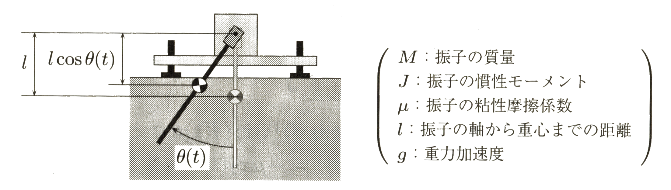
Figure 5 Pendulum system with parameters
Let , denote the state variables. Then equation (2) is rewritten as
Equilibrium point is obtained as
Therefore, is one of the Equilibrium point . Besides, the mechanical energy of pendulum system equation (3) is
where the first term at right hand is called kinetic energy , the second one is called potential energy as is shown in Figure 6
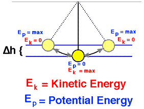
Figure 6 Mechanical energy of pendulum
When , that the position of pendulum is six o'clock, and velocity of it is 0, then . For any other state there is . The derivative of with equation (3) as simultaneous equations in order to cancel derivatives of states, the following formula holds as
Assume
| ( moment of inertia ) | |||
|---|---|---|---|
| 1 | 1 | 1 | 1 |
Matlab code of machanical energy is:
                                [X,Y] = meshgrid(-7:0.1:7,-10:0.1:10);
    Z = Y.^2 + 9.8*(1-cos(X));
    surf(X,Y,Z)
    xlabel('angle')
    ylabel('angular velocity')

Figure 7 Mechanical energy of pendulum (Matlab chart)
Matlab code of is:
                                [X,Y] = meshgrid(-7:0.1:7,-10:0.1:10);
    Z = -Y.^2;
    surf(X,Y,Z)
    xlabel('angle')
    ylabel('angular velocity')

Figure 8 Derivative of pendulum mechanical energy (Matlab chart)
Note that is a positive-definite function (PDF), ( ), while . Unlike single-variable functions, whose time-derivatives indicate monotonicity, multi-variable function as shown in equation (5) , whose time-derivative is utilized to exploit the stability of an equilibrium point. [ref] Generally,
which in a scalar (dot) product can be written as
Here, the first vector is the gradient of , id est, it’s always directed toward the greatest increase in . The second vector is velocity vector, it is always tagent to the phase trajectory .

(a)

(b)
Figure 9 (a) Lyapunov function. (b) Phase trajectory.
Take pendulum system equation (3) again for example, the gradient and phase trajectory of which is obtained by Matlab code as below [ref] :
                                            x=-pi:pi/20:pi;
    y=x';
    z = y.^2 + 9.8*(1-cos(x));
    [px,py] = gradient(z);
    figure
    contour(x,y,z)
    hold on
    quiver(x,y,px,py)
    hold off
    xlabel('angle')
    ylabel('angular velocity')
                                            x=-pi:pi/20:pi;
    y=x';
    z = y.^2 + 9.8*(1-cos(x));
    vx = y*ones(1,41);
    vy=-9.8*sin(x)-y*ones(1,41);
    figure
    contour(x,y,z)
    hold on
    quiver(x,y,vx,vy)
    hold off
    xlabel('angle')
    ylabel('angular velocity')

(a)

(b)
Figure 10 (a) Gradient chart. (b) Phase trajectory chart.
For phase trajectory and state trajectory of system (2) [ref] [ref] [ref] [ref]
                                syms x(t)
    [V] = odeToVectorField(diff(x, 2) == -diff(x,1) - 9.8*sin(x));
    M = matlabFunction(V,'vars', {'t','Y'});
    sol = ode45(M,[0 20],[2 2]);
    z = linspace(0,20,1000);
    x1 = deval(sol,z,1);
    x2 = deval(sol,z,2);
    figure
    hold on;
    plot(x1,x2);
    xlabel('angle')
    ylabel('angular velocity')
    hold off;
    figure
    hold on;
    fplot(@(x)deval(sol,x,1), [0, 20])
    xlabel('time')
    ylabel('angle')
    hold off;
    figure
    hold on;
    fplot(@(x)deval(sol,x,2), [0, 20])
    xlabel('time')
    ylabel('angular velocity')
    hold off;

Figure 11 Phase portrait

Figure 12(a) angle trajectory

Figure 12(b) angular velocity trajectory
Test initial condition for
[5,5],[3.14,5],[3.14,0],[3.14,-5],[pi,0].
Back to
equation (6)
, when
, if
, there are chances that
is stable. Whatsoever,
When
, then
. Such that,
, when
. Therefore, such "equilibriums" are not stable.
Figure (13)
and
figure (14)
represent
mechnical energy
of pendulum system
(2)
and its time derivatives respectively. The matlab code is
    ...
    fplot(@(x) 0.5*deval(sol,x,2).^2+9.8-9.8*cos(deval(sol,x,1)), [0, 20])
    fplot(@(x) -deval(sol,x,2).^2, [0, 20])
Figure 13
