Paper Z
Packet dropout prevention in networked control systems based on model predictive control approach
References
→ overall
モデル予測制御
Minimax approaches to robust model predictive control
→ Kalman filter
Understanding and Applying Kalman Filtering
Kalman Filtering - Theory and Practice Using MATLAB
Digital Control of Dynamic Systems
Tutorial - The Kalman Filter
the Kalman filter
MIT- Kalman Filter
Issues
→ Kalman filter
1. staffs
1.1 materials
- book page 278, or pdf page 148 of モデル予測制御, a well interpreted version of Kalman filter in Japanese briefly
- Understanding and Applying Kalman Filtering, some easiest concept
- Kalman Filtering - Theory and Practice Using MATLAB, Matlab realization
- book page 389, or pdf page 205 of Digital Control of Dynamic Systems, original algorithm
- page 5~6 of Tutorial - The Kalman Filter, algorithm
- MIT- Kalman Filter
- Matlab introduction of Kalman filter
- Kalman filter design by Matlab
1.2 codes
1.3 GitHub assembly
https://github.com/Trancemania/Kalman-filter/tree/origin
2. pre-knowledge
2.1 objective
Theoretically, the Kalman filter is an estimator for what is called the linear-quadratic problem. [kf1]EXAMPLE 1: continuous-time plant model Kalman filter
(kf.1)
with , is thestandard deviation, or square root ofvarianceof white noisenormal distribution, and is theexpectationoperator. [kf2] [kf3] [kf4] [kf5]
A typical Kalman filter design can be demonstrated as:
where Kalman filter gain [kf6] is the variable needs to be worked out. The system in Fig. kf1 can be described as: 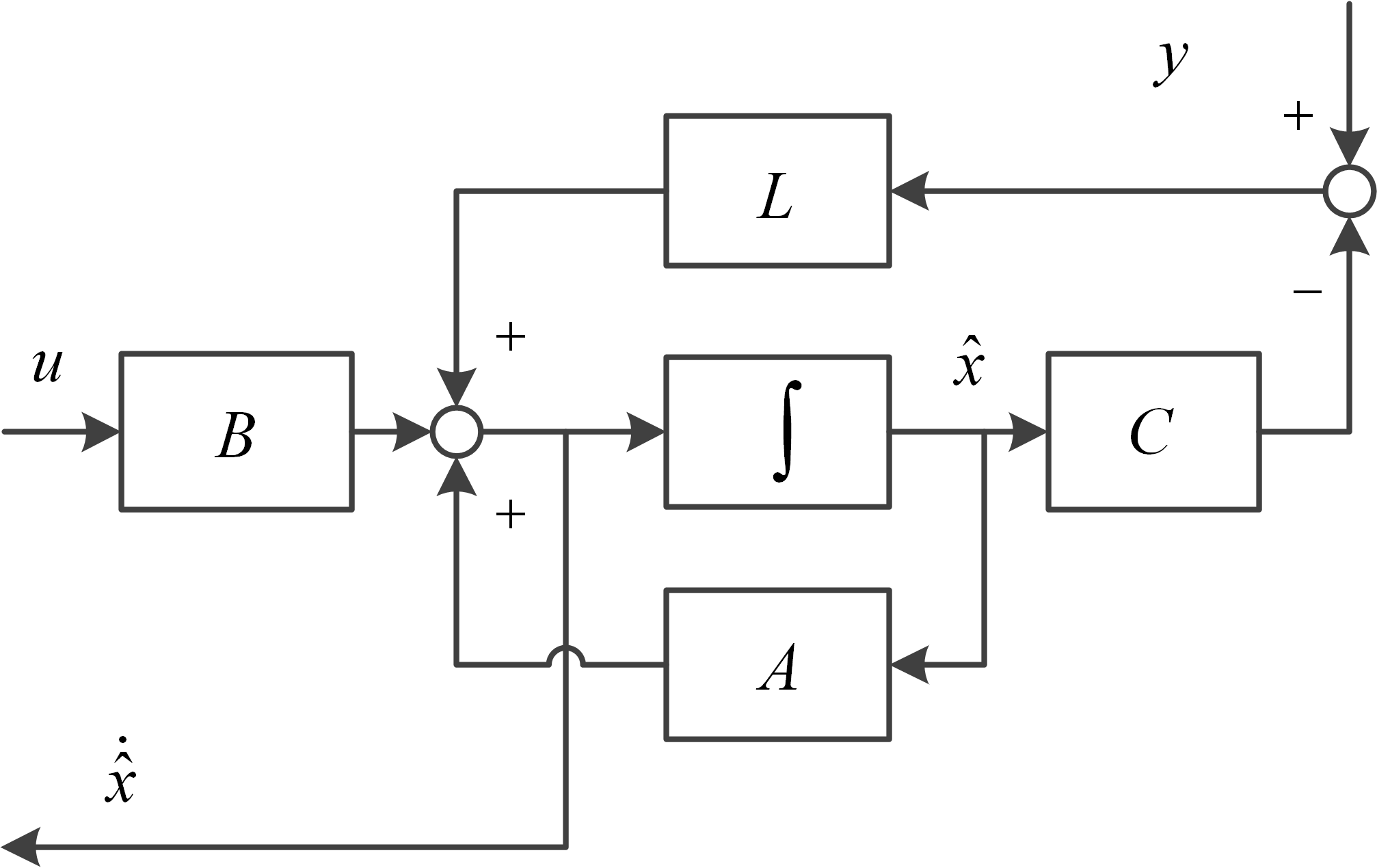
Fig. kf1 continuous Kalman filter design [source file]
(kf.2)
where is the estimate of system state .
Theestimation errormay be defined as , thus, [kf7]
\begin{aligned} \dot{\boldsymbol{e}}&=(\boldsymbol{A}\boldsymbol{x}+\boldsymbol{B}\boldsymbol{u}+\boldsymbol{\omega})-[\boldsymbol{A}\widehat{\boldsymbol{x}}+\boldsymbol{B}\boldsymbol{u}+\boldsymbol{L}(\boldsymbol{y}-\boldsymbol{C}\widehat{\boldsymbol{x}})]\\ &= (\boldsymbol{A}-\boldsymbol{L}\boldsymbol{C})\boldsymbol{e}+(\boldsymbol{\omega}-\boldsymbol{L}\boldsymbol{\nu}) \end{aligned} (kf.3)
Kalman filter design provides that minimizes the scalarcost function[kf8]
(kf.4)
where is an unspecified symmetric, positive definite weighting matrix, which penalize specified state(in this case) [kf9] [kf10] . A related matrix, the symmetricerror covariance, is defined as
(kf.5)
Notice that is a matrix.
Further reading about matrix, vector, derivative, calculus, quadratic forms, , .
A general solution of (kf.3) may be written as [kf11] [kf12] [kf13] :(kf.6)
Thus,\begin{aligned} \dot{\boldsymbol\Sigma}&=\mathrm E(\dot{\boldsymbol e}\boldsymbol e^T+\boldsymbol e\dot{\boldsymbol e}^T)\\&=\mathrm E[(\boldsymbol{A}-\boldsymbol{L}\boldsymbol{C})\boldsymbol{e}\boldsymbol e^T+(\boldsymbol{\omega}-\boldsymbol{L}\boldsymbol{\nu})\boldsymbol e^T+\boldsymbol{e}\boldsymbol e^T(\boldsymbol{A}^T-\boldsymbol{C}^T\boldsymbol{L}^T)+\boldsymbol e(\boldsymbol{\omega}^T-\boldsymbol{\nu}^T\boldsymbol{L}^T)] \end{aligned} (kf.7)
by substitution of (kf.6) into (kf.7) , the final expression of which may be rewritten into\begin{aligned} \mathrm E [\boldsymbol{e}(\boldsymbol{\omega}^T-\boldsymbol{\nu}^T\boldsymbol{L}^T)]&=\mathrm{e}^{(\boldsymbol{A}-\boldsymbol{LC})t}\mathrm E [\boldsymbol{e}(0)(\boldsymbol{\omega}^T-\boldsymbol{\nu}^T\boldsymbol{L}^T)]\\&+\int_0^t\mathrm e^{(\boldsymbol A-\boldsymbol L\boldsymbol C)(t-\tau)}\mathrm E\lbrack(\boldsymbol{\omega}^T(t)-\boldsymbol{\nu}^T(t)\boldsymbol{L}^T)(\boldsymbol\omega(\tau)-\boldsymbol L\boldsymbol\nu(\tau)\rbrack\mathrm d\tau \end{aligned} (kf.8)
Notice that the initial condition is uncorrelated with , therefore,(kf.9)
By reasoning process in book page 20 or pdf page 3 of MIT- Kalman Filter , (kf.8) may be reformed into(kf.10)
According to page 9 theorem 1.5 of [kf14] , and [kf15] [kf16] [kf17] , (kf.4) may be rewritten as(kf.11)
An auxiliary cost function may be introduced and defined as(kf.12)
where is an matrix of zeros, and is an matrix of unknown Lagrange multiplier [kf18] , which provide an ingenious mechanism for drawing constraints into the optimization. In this case, is designed as(kf.13)
Riccati average model ref3