Chapter 1: 古典制御理論から現代制御理論へ
→ 1.1高次システムに対する古典制御理論の限界
例1.1 transfer function representation
example1_1.m
                        syms s y u z
eq1 = 0.5*s^2*z==u-2*(z-y)-(s*z-s*y);
eq2 = s^2*y==2*(z-y)+(s*z-s*y);         %input simultaneous equations

cancelZ = solve(eq2, z);                %cancel Z from eq2
uy = subs(eq1, z, cancelZ);             %substitute Z into eq1
Ps = subs(solve(uy, y),u,1);            %symbolic transfer function
[symnum,symden] = numden(Ps);           %extract num den
num = sym2poly(symnum);
den = sym2poly(symden);                 %matrix format

tf = tf(num,den);                       %transfer function
%num = cell2mat(tf.numerator(1,1));
%den = cell2mat(tf.denominator(1,1));   %cell to matrix
example1_1.m
shows how to generate transfer function from frequency domain equations (1.1)
例1.2 process variable derivative controller
PD_controller.slx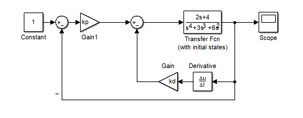
Figure 1.1 PD process variable derivative controller
                        % run example1_1.m first
syms x
Px = poly2sym(num,x)/poly2sym(den,x);                               %symbolic transfer function with variable x
syms kpx kdx
Ts = Px*kpx/(1+Px*(kdx*x+kpx));                                     %close-loop transfer function with PD controller
invTs_bar = taylor(1/Ts, x, 0, 'Order', 4);                         %taylor series of first three terms
syms wn ksi
GMx = wn^2/(x^2+2*ksi*wn*x+wn^2);                                   %normal model transfer function
para_invGMs = coeffs(1/GMx, x, 'All');                              %symbolic coefficiets in matrix format
para_invTs_bar = coeffs(invTs_bar, x, 'All');                       %symbolic coefficiets in matrix format
[kpsol,kdsol] = solve(para_invGMs == para_invTs_bar, [kpx,kdx]);    %solve
kp = double(subs(kpsol, [wn ksi], [0.5 0.7]));                      %numeric substitution sym2mat
kd = double(subs(kdsol, [wn ksi], [0.5 0.7]));                      %numeric substitution sym2mat
example1_2.m
shows how to calculate portion parameter
and differential parameter
according to specified damping rate
and natural frequency
for a high order system in
Fig. 1.1
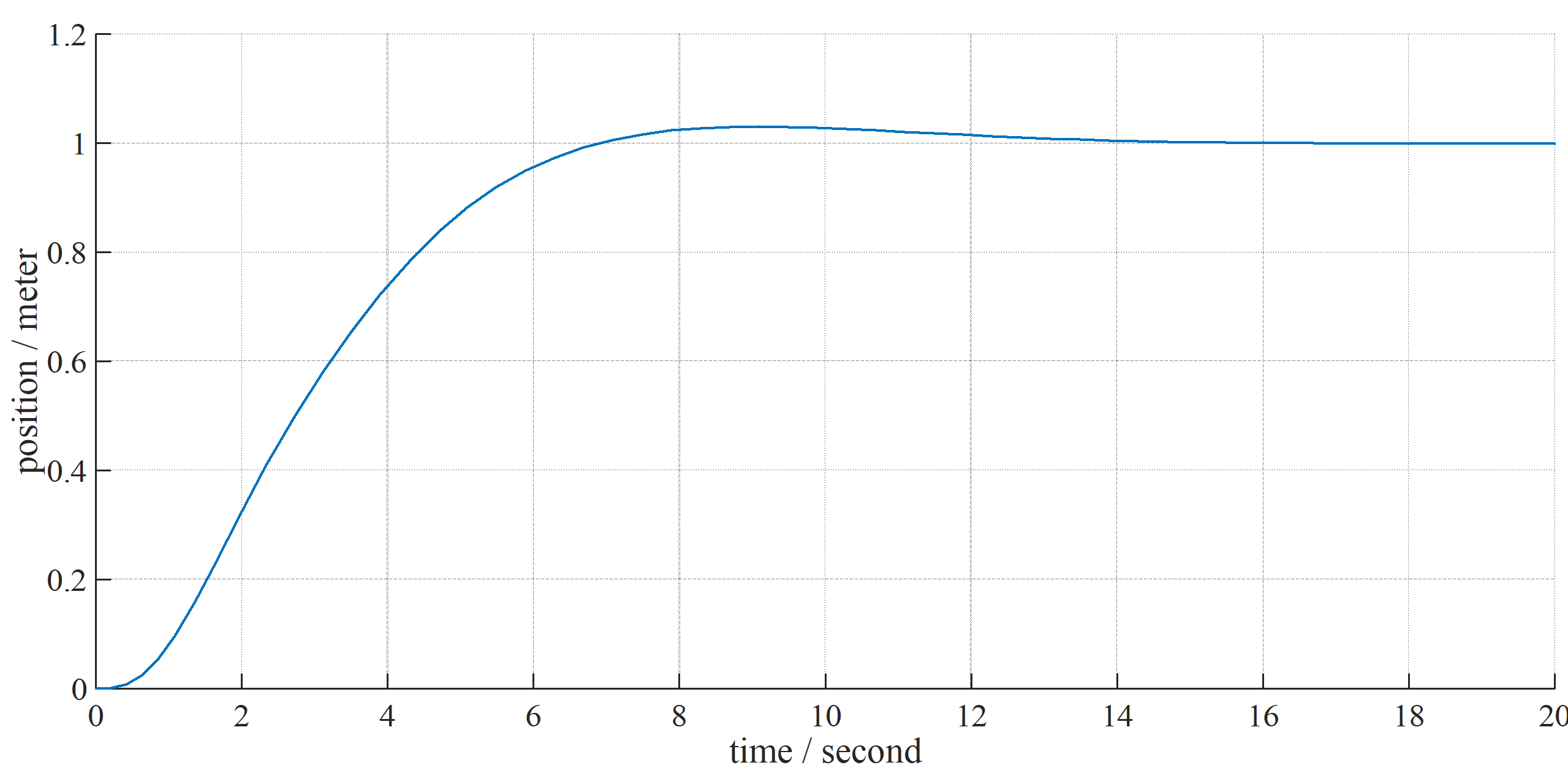
Figure 1.2 simulation result of PD controller in example1_2.m with and
→ 1.2現代制御理論における高次システムの取り扱い
例1.3 state feedback control
This example shows the relevance between state feedback and process variable derivative.The process variable derivative control in Fig. 1.1 can be rewritten as
where in Eq. 1.1.
When taking account of , a new process variable derivative controller may be proposed as
example1_3.slx
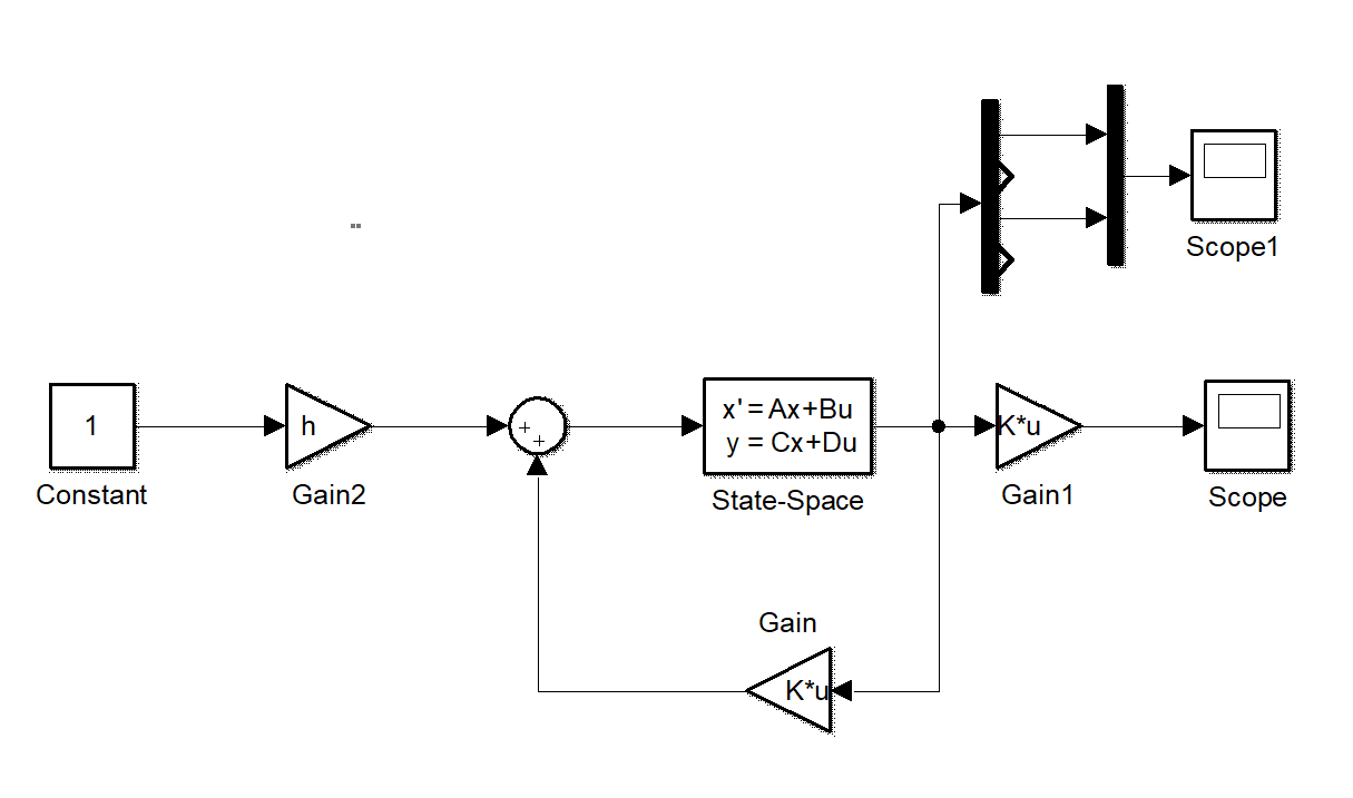
Figure 1.3 state feedback controller
                        % run example1_1.m first
%% transfer function
syms kp1 kp2 kd1 kd2 yref
us2 = kp1*(yref-cancelZ)-kd1*s*cancelZ+kp2*(yref-y)-kd2*s*y;        %control input
close_loop2 = us2*Ps==y;                                            %close loop
Ts2 = subs(solve(close_loop2, y),yref,1);                           %transfer function
[symnum2,symden2] = numden(Ts2);                                    %extract num den
num2 = coeffs(symnum2, s, 'All');
den2 = coeffs(symden2, s, 'All');                                   %coefficients of s

ss_Ps = ss(tf);                                                     %derive A,B,C matrix for simulation
                        %WARNING:ss_Ps is not suitable for
                        %simulation 1_3 since states change,

k = [-1.9, -1.71, -5.84, -4.45];                                    %controller gains from book
h = 7.75;

A = [0 1 0 0;-4 -2 4 2;0 0 0 1;2 1 -2 -1];                          %A,B,C matrix by input
B = [0;2;0;0];
C = [0,0,1,0];
E: ss_Ps in
example1_3.m
mustn't be used in
example1_3.slx
as State-Space shown in
Fig. 1.3
, since states change in the process of tf2ss.
In order to set state-space parameters correctly, example1_3_sup.m is proposed.
                        % this supplyment shows how to generate state space from differential equations
syms x1(t) x2(t) x3(t) x4(t) u;

eqs = [diff(x1(t),t) == x2(t),...
       0.5*diff(x2(t),t) == -2*(x1(t)-x3(t))-(x2(t)-x4(t))+u,...
       diff(x3(t),t) == x4(t),...
       diff(x4(t),t) == 2*(x1(t)-x3(t))+(x2(t)-x4(t))];
[vf,Yvar] = odeToVectorField(eqs);                                  % ODE to vector field

rearr = matlabFunction(Yvar);
x_state_rearr = rearr(x1,x2,x3,x4);
x_state = [x1;x2;x3;x4];
[i,j] = find(x_state*transpose(1./x_state_rearr)==1);
TrM = zeros(4);
TrM(sub2ind([4,4],i,j)) = 1;                                        %since odeToVectorField rearrange states, this
                        %step gets transformation matrix to arrange
                        %correctly
sort_vf = TrM*vf;
F_vf = matlabFunction(sort_vf);
x_vf = F_vf(Yvar,u);
mat_A = double(equationsToMatrix(x_vf ==0, TrM*Yvar));
mat_B = double(equationsToMatrix(x_vf ==0, u));

mat_C = [0 0 1 0];                                                  %use new syms and equationsToMatrix when complicated
mat_A
,
mat_B
and
mat_C
are the corresponding parameters in
Fig. 1.3
. The controller parameters
and
in
Fig. 1.3
and
Eq. 1.3
may be derived by minimizing cost function
According to N: optimal regulator theory , the result of optimization Eq. 1.4 is
Q: How to derive the result of Eq. 1.5 .
The simulation results of Fig. 1.3 with Eq. 1.5 and mat_A , mat_B , mat_C in example1_3_sup.m are shown below.
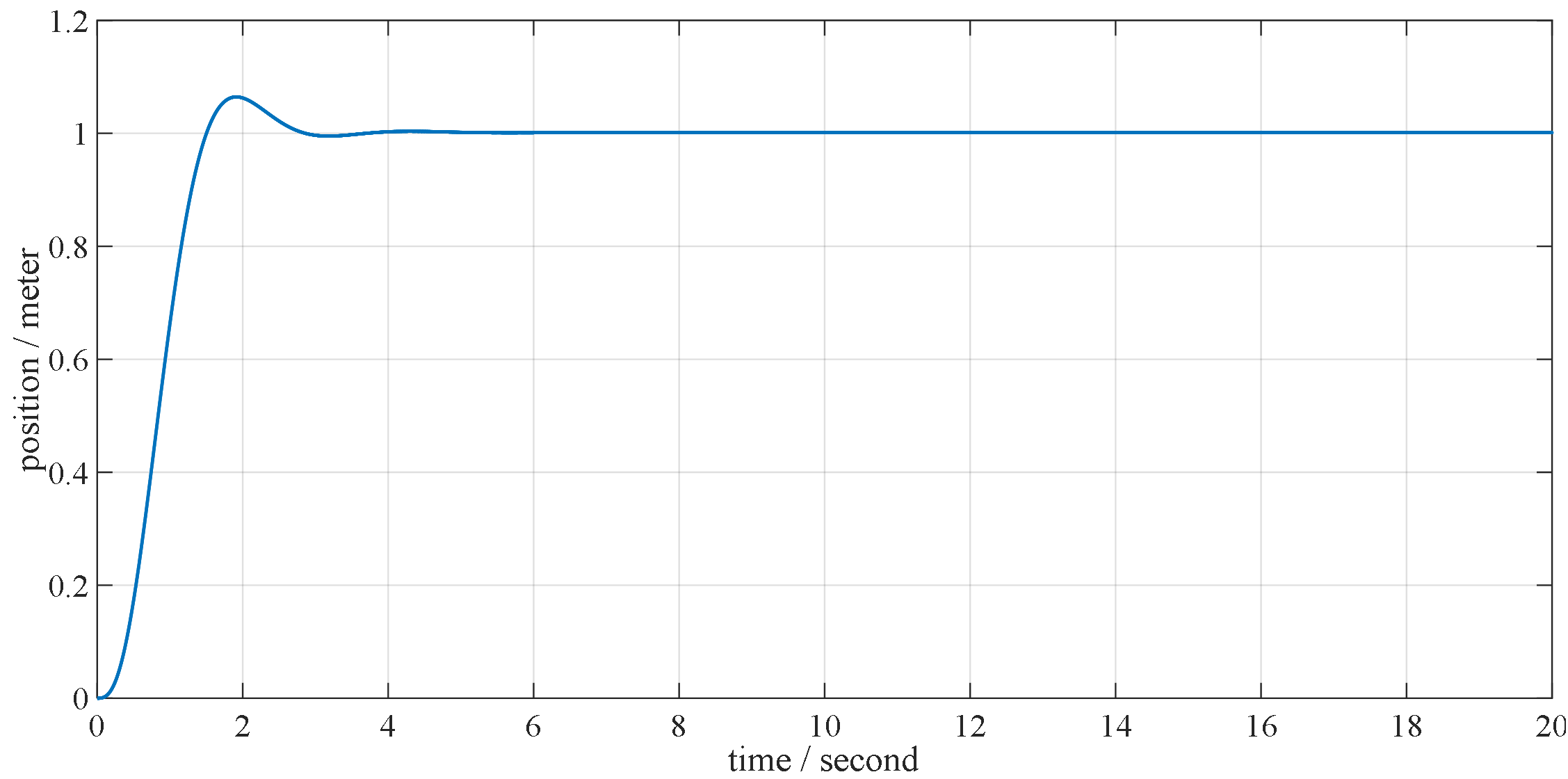
a) simulation result of output
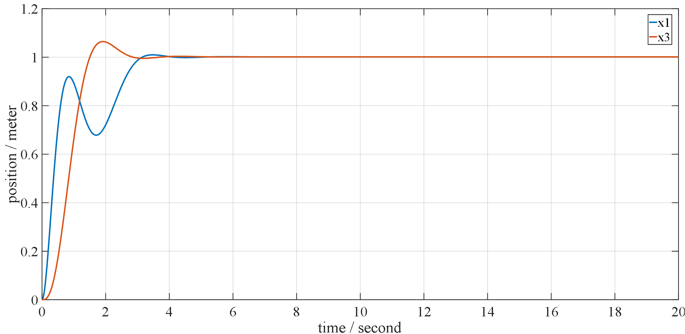
b) simulation result of states
Figure 1.4 simulation results of Fig. 1.3 under condition of example1_3_sup.m and Eq. 1.5
example1_3_control.slx
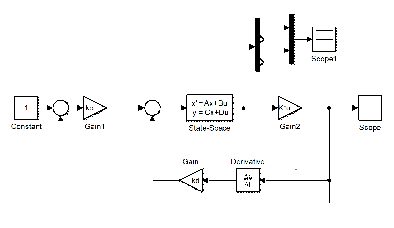
Figure 1.5 the state-space form of Fig. 1.1
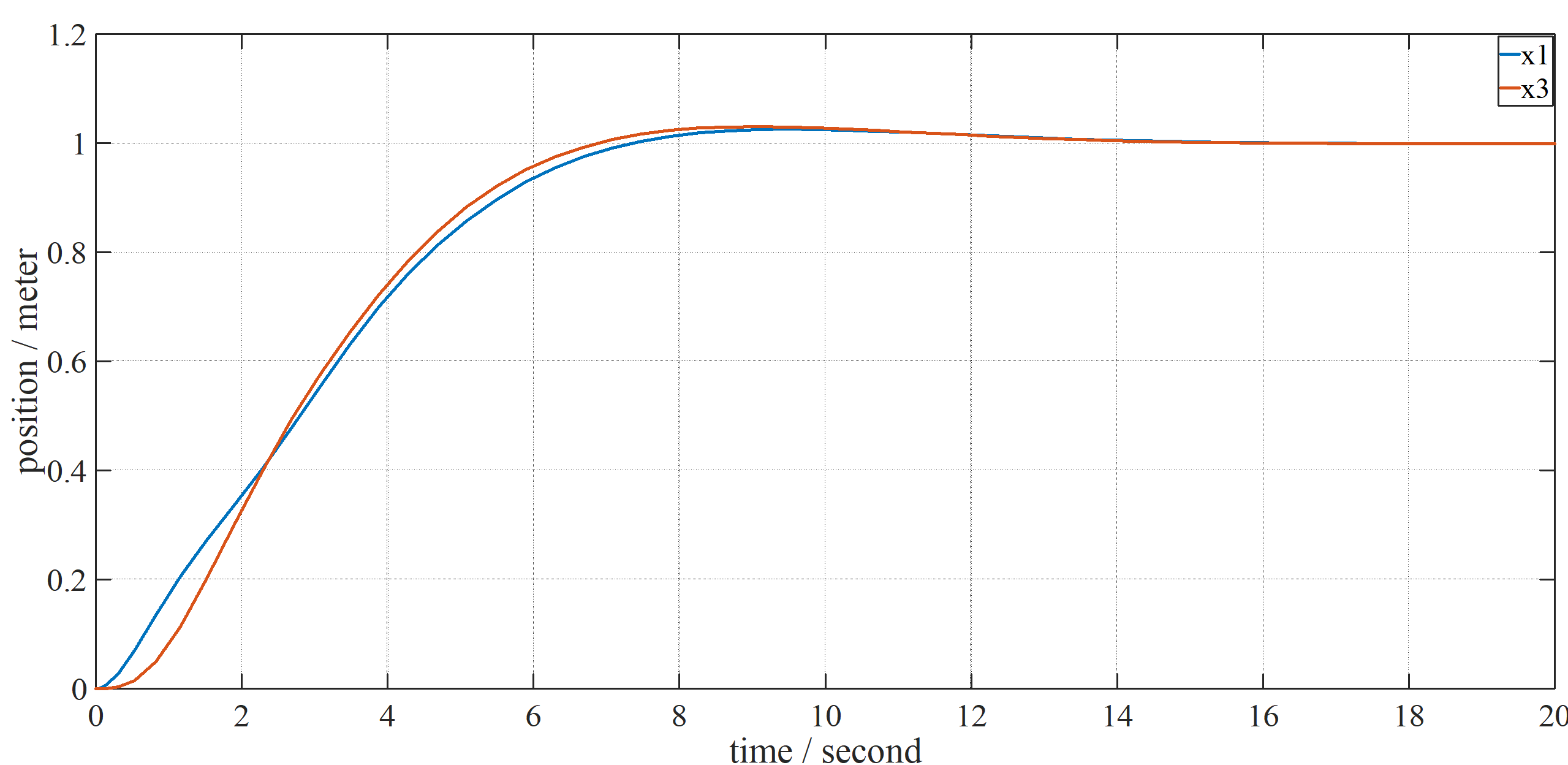
Figure 1.6 waveforms of states in Fig. 1.5
We also present another control group of common PD controller. The brief diagram is shown below.
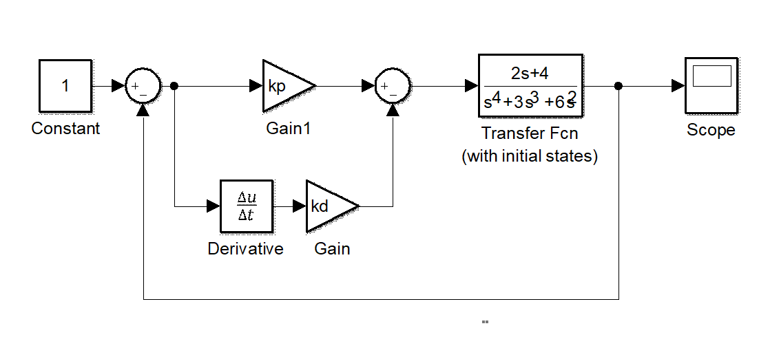
Figure 1.7 brief diagram of common PD controller
                        % run example1_1.m first
syms kpp kdd yref
eq3 = y == Ps*kpp*(yref-y)+kdd*s*(yref-y);
tf_pd = subs(solve(eq3, y),yref,1);
[sym_pd_num,sym_pd_den] = numden(tf_pd);
pd_num = coeffs(sym_pd_num, s, 'All');
pd_den = coeffs(sym_pd_den, s, 'All');

tl4 = taylor(1/tf_pd, s, 0, 'Order', 4);
tl5 = taylor(1/tf_pd, s, 0, 'Order', 5);
tl6 = taylor(1/tf_pd, s, 0, 'Order', 6);
By calculating 3rd to 6th order taylor series as tl4,
tl5
and
tl6
in
normal_pd.m
, the result shows that
derivative gain
only appears in taylor series with order higher than 5, which means derivative gain in common PD controller has little influence on such high order target plant with transfer function
Ps
in
example1_1.m
.
→ 1.3多入力多出力システムに対する古典制御理論の限界
例1.4 2 inputs 2 outputs transfer function representation
example1_4.m
                        %% MIMO state space
syms x1(t) x2(t) x3(t) x4(t) u1 u2;

eqs = [diff(x1(t),t) == x2(t),...
       0.5*diff(x2(t),t) == -2*(x1(t)-x3(t))-(x2(t)-x4(t))+u1,...
       diff(x3(t),t) == x4(t),...
       diff(x4(t),t) == 2*(x1(t)-x3(t))+(x2(t)-x4(t))+u2];
[vf,Yvar] = odeToVectorField(eqs);
rearr = matlabFunction(Yvar);
x_state_rearr = rearr(x1,x2,x3,x4);
x_state = [x1;x2;x3;x4];
[i,j] = find(x_state*transpose(1./x_state_rearr)==1);
TrM = zeros(4);
TrM(sub2ind([4,4],i,j)) = 1;

sort_vf = TrM*vf;
F_vf = matlabFunction(sort_vf);
x_vf = F_vf(Yvar,u1,u2);
mat_A = double(equationsToMatrix(x_vf ==0, TrM*Yvar));
mat_B = double(equationsToMatrix(x_vf ==0, [u1,u2]));
mat_C = [1 0 0 0; 0 0 1 0];

%% MIMO transfer function
syms y1 y2 s;
eq1 = 0.5*s^2*y1==u1-2*(y1-y2)-(s*y1-s*y2);
eq2 = s^2*y2==u2+2*(y1-y2)+(s*y1-s*y2);
cancely1 = solve(eq2, y1);
uy1 = subs(eq1, y1, cancely1);
tf_y1u1 = subs(solve(uy1, y2),[u1,u2],[1,0]);
tf_y1u2 = subs(solve(uy1, y2),[u1,u2],[0,1]);

cancely2 = solve(eq2, y2);
uy2 = subs(eq1, y2, cancely2);
tf_y2u1 = subs(solve(uy2, y1),[u1,u2],[1,0]);
tf_y2u2 = subs(solve(uy2, y1),[u1,u2],[0,1]);

mat_tf = [tf_y1u1, tf_y1u2; tf_y2u1, tf_y2u2];
Control of an MIMO system based on transfer function representation requires an approximation to decouple the transfer function matrix, even though, there
still exists interference between inputs and outputs. While control method based on state-space representation has no such worry.
Q: optimal regulator theory solved example 1.6